Computing LLPR uncertainties

This tutorial demonstrates how to use an already trained and exported model from Python. It involves the computation of the local prediction rigidity (LPR) for every atom of a single ethanol molecule, using the last-layer prediction rigidity (LLPR) approximation.

The model was trained using the following training options.

device: cpu
base_precision: 64
seed: 42

architecture:
  name: soap_bpnn
  training:
    batch_size: 16
    num_epochs: 10
    learning_rate: 0.01

# Section defining the parameters for system and target data
training_set:
  systems: "qm9_reduced_100.xyz"
  targets:
    energy:
      key: "U0"
      unit: "hartree"  # very important to run simulations

validation_set: 0.1
test_set: 0.0

You can train the same model yourself with

#!/bin/bash

mtt train options.yaml

A detailed step-by-step introduction on how to train a model is provided in the Basic Usage tutorial.

import torch

from metatrain.utils.io import load_model

Models can be loaded using the metatrain.utils.io.load_model() function from the. For already exported models The function requires the path to the exported model and, for many models, also the path to the respective extensions directory. Both are produced during the training process.

model = load_model("model.pt", extensions_directory="extensions/")

In metatrain, a Dataset is composed of a list of systems and a dictionary of targets. The following lines illustrate how to read systems and targets from xyz files, and how to create a Dataset object from them.

from metatrain.utils.data import Dataset, read_systems, read_targets  # noqa: E402
from metatrain.utils.neighbor_lists import (  # noqa: E402
    get_requested_neighbor_lists,
    get_system_with_neighbor_lists,
)


qm9_systems = read_systems("qm9_reduced_100.xyz")

target_config = {
    "energy": {
        "quantity": "energy",
        "read_from": "ethanol_reduced_100.xyz",
        "reader": "ase",
        "key": "energy",
        "unit": "kcal/mol",
        "type": "scalar",
        "per_atom": False,
        "num_subtargets": 1,
        "forces": False,
        "stress": False,
        "virial": False,
    },
}
targets, _ = read_targets(target_config)

requested_neighbor_lists = get_requested_neighbor_lists(model)
qm9_systems = [
    get_system_with_neighbor_lists(system, requested_neighbor_lists)
    for system in qm9_systems
]
dataset = Dataset.from_dict({"system": qm9_systems, **targets})

# We also load a single ethanol molecule on which we will compute properties.
# This system is loaded without targets, as we are only interested in the LPR
# values.
ethanol_system = read_systems("ethanol_reduced_100.xyz")[0]
ethanol_system = get_system_with_neighbor_lists(
    ethanol_system, requested_neighbor_lists
)

The dataset is fully compatible with torch. For example, be used to create a DataLoader object.

from metatrain.utils.data import collate_fn  # noqa: E402


dataloader = torch.utils.data.DataLoader(
    dataset,
    batch_size=10,
    shuffle=False,
    collate_fn=collate_fn,
)

We now wrap the model in a LLPRUncertaintyModel object, which will allows us to compute prediction rigidity metrics, which are useful for uncertainty quantification and model introspection.

from metatensor.torch.atomistic import (  # noqa: E402
    MetatensorAtomisticModel,
    ModelMetadata,
)

from metatrain.utils.llpr import LLPRUncertaintyModel  # noqa: E402


llpr_model = LLPRUncertaintyModel(model)
llpr_model.compute_covariance(dataloader)
llpr_model.compute_inverse_covariance(regularizer=1e-4)

# calibrate on the same dataset for simplicity. In reality, a separate
# calibration/validation dataset should be used.
llpr_model.calibrate(dataloader)

exported_model = MetatensorAtomisticModel(
    llpr_model.eval(),
    ModelMetadata(),
    llpr_model.capabilities,
)

We can now use the model to compute the LPR for every atom in the ethanol molecule. To do so, we create a ModelEvaluationOptions object, which is used to request specific outputs from the model. In this case, we request the uncertainty in the atomic energy predictions.

from metatensor.torch.atomistic import ModelEvaluationOptions, ModelOutput  # noqa: E402


evaluation_options = ModelEvaluationOptions(
    length_unit="angstrom",
    outputs={
        # request the uncertainty in the atomic energy predictions
        "energy": ModelOutput(per_atom=True),  # needed to request the uncertainties
        "mtt::aux::energy_uncertainty": ModelOutput(per_atom=True),
        # `per_atom=False` would return the total uncertainty for the system,
        # or (the inverse of) the TPR (total prediction rigidity)
        # you also can request other outputs from the model here, for example:
        # "mtt::aux::energy_last_layer_features": ModelOutput(per_atom=True),
    },
    selected_atoms=None,
)

outputs = exported_model([ethanol_system], evaluation_options, check_consistency=False)
lpr = outputs["mtt::aux::energy_uncertainty"].block().values.detach().cpu().numpy()

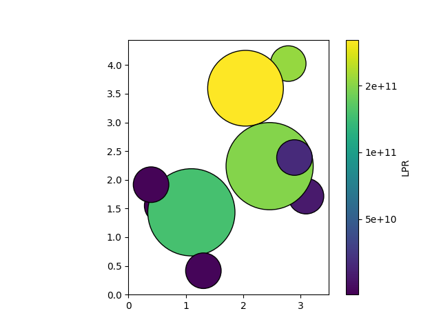
We can now visualize the LPR values using the plot_atoms function from ase.visualize.plot.

import ase.io  # noqa: E402
import matplotlib.pyplot as plt  # noqa: E402
from ase.visualize.plot import plot_atoms  # noqa: E402
from matplotlib.colors import LogNorm  # noqa: E402


structure = ase.io.read("ethanol_reduced_100.xyz")
norm = LogNorm(vmin=min(lpr), vmax=max(lpr))
colormap = plt.get_cmap("viridis")
colors = colormap(norm(lpr))
ax = plot_atoms(structure, colors=colors, rotation="180x,0y,0z")
custom_ticks = [1e10, 2e10, 5e10, 1e11, 2e11]
cbar = plt.colorbar(
    plt.cm.ScalarMappable(norm=norm, cmap=colormap),
    ax=ax,
    label="LPR",
    ticks=custom_ticks,
)
cbar.ax.set_yticklabels([f"{tick:.0e}" for tick in custom_ticks])
cbar.minorticks_off()
plt.show()