Running molecular dynamics with ASE

This tutorial demonstrates how to use an already trained and exported model to run an ASE simulation of a single ethanol molecule in vacuum. We use a model that was trained using the SOAP-BPNN architecture on 100 ethanol systems containing energies and forces. You can obtain the dataset file used in this example from our website. The dataset is a subset of the rMD17 dataset.

The model was trained using the following training options.

seed: 42

architecture:
  name: gap

# training set section
training_set:
  systems: "ethanol_reduced_100.xyz"
  targets:
    energy:
      key: "energy"
      unit: "kcal/mol" # very important to run simulations

validation_set: 0.1
test_set: 0.0

You can train the same model yourself with

#!/bin/bash

mtt train options.yaml

A detailed step-by-step introduction on how to train a model is provided in the Basic Usage tutorial.

First, we start by importing the necessary libraries, including the integration of ASE calculators for metatensor atomistic models.

import ase.md
import ase.md.velocitydistribution
import ase.units
import ase.visualize.plot
import matplotlib.pyplot as plt
import numpy as np
from ase.geometry.analysis import Analysis
from metatensor.torch.atomistic.ase_calculator import MetatensorCalculator

Setting up the simulation

Next, we initialize the simulation by extracting the initial positions from the dataset file which we initially trained the model on.

train_frames = ase.io.read("ethanol_reduced_100.xyz", ":")
atoms = train_frames[0].copy()

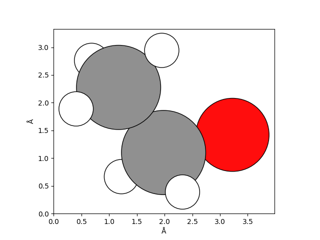
Below we show the initial configuration of a single ethanol molecule in vacuum.

ase.visualize.plot.plot_atoms(atoms)

plt.xlabel("Å")
plt.ylabel("Å")

plt.show()

Our initial coordinates do not include velocities. We initialize the velocities according to a Maxwell-Boltzmann Distribution at 300 K.

ase.md.velocitydistribution.MaxwellBoltzmannDistribution(atoms, temperature_K=300)

We now register our exported model as the energy calculator to obtain energies and forces.

atoms.calc = MetatensorCalculator("model.pt", extensions_directory="extensions/")

the model suggested to use CUDA devices before CPU, but we are unable to find it

Finally, we define the integrator which we use to obtain new positions and velocities based on our energy calculator. We use a common timestep of 0.5 fs.

integrator = ase.md.VelocityVerlet(atoms, timestep=0.5 * ase.units.fs)

Run the simulation

We now have everything ready to run the MD simulation at constant energy (NVE). To keep the execution time of this tutorial small we run the simulations only for 100 steps. If you want to run a longer simulation you can increase the n_steps variable.

During the simulation loop we collect data about the simulation for later analysis.

n_steps = 100

potential_energy = np.zeros(n_steps)
kinetic_energy = np.zeros(n_steps)
total_energy = np.zeros(n_steps)
trajectory = []

for step in range(n_steps):
    # run a single simulation step
    integrator.run(1)

    trajectory.append(atoms.copy())
    potential_energy[step] = atoms.get_potential_energy()
    kinetic_energy[step] = atoms.get_kinetic_energy()
    total_energy[step] = atoms.get_total_energy()

Analyse the results

Energy conservation

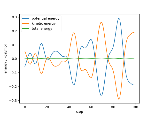
For a first analysis, we plot the evolution of the mean of the kinetic, potential, and total energy which is an important measure for the stability of a simulation.

As shown below we see that both the kinetic, potential, and total energy fluctuate but the total energy is conserved over the length of the simulation.

plt.plot(potential_energy - potential_energy.mean(), label="potential energy")
plt.plot(kinetic_energy - kinetic_energy.mean(), label="kinetic energy")
plt.plot(total_energy - total_energy.mean(), label="total energy")

plt.xlabel("step")
plt.ylabel("energy / kcal/mol")
plt.legend()

plt.show()

Inspect the systems

Even though the total energy is conserved, we also have to verify that the ethanol molecule is stable and the bonds did not break.

animation = ase.visualize.plot.animate(trajectory, interval=100, save_count=None)
plt.show()

Once Loop Reflect

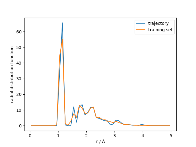
Carbon-hydrogen radial distribution function

As a final analysis we also calculate and plot the carbon-hydrogen radial distribution function (RDF) from the trajectory and compare this to the RDF from the training set.

To use the RDF code from ase we first have to define a unit cell for our systems. We choose a cubic one with a side length of 10 Å.

for atoms in train_frames:
    atoms.cell = 10 * np.ones(3)
    atoms.pbc = True

for atoms in trajectory:
    atoms.cell = 10 * np.ones(3)
    atoms.pbc = True

We now can initilize the ase.geometry.analysis.Analysis objects and compute the the RDF using the ase.geometry.analysis.Analysis.get_rdf() method.

ana_traj = Analysis(trajectory)
ana_train = Analysis(train_frames)

rdf_traj = ana_traj.get_rdf(rmax=5, nbins=50, elements=["C", "H"], return_dists=True)
rdf_train = ana_train.get_rdf(rmax=5, nbins=50, elements=["C", "H"], return_dists=True)

We extract the bin positions from the returned values and and averege the RDF over the whole trajectory and dataset, respectively.

bins = rdf_traj[0][1]
rdf_traj_mean = np.mean([rdf_traj[i][0] for i in range(n_steps)], axis=0)
rdf_train_mean = np.mean([rdf_train[i][0] for i in range(n_steps)], axis=0)

Plotting the RDF verifies that the hydrogen bonds are stable, confirming that we performed an energy-conserving and stable simulation.

plt.plot(bins, rdf_traj_mean, label="trajectory")
plt.plot(bins, rdf_train_mean, label="training set")

plt.legend()
plt.xlabel("r / Å")
plt.ylabel("radial distribution function")

plt.show()