Splined radial integral

This examples shows how to feed custom radial integrals (as splines) to the Rust calculators that use radial integrals: the SOAP and LODE spherical expansions, and any other calculator based on these.

Python

This example illustrates how to generate splines and use custom basis function and density when computing density-based representations, such as SOAP or LODE.

import json

import ase.build
import matplotlib.pyplot as plt
import numpy as np
import scipy

import featomic
from featomic import SphericalExpansion
from featomic.basis import RadialBasis
from featomic.splines import SoapSpliner

For this example, we will define a new custom radial basis for the SOAP spherical expansion, based on Chebyshev polynomials of the first kind. This basis will then be used in combination with spherical harmonics to expand the density of neighboring atoms around a central atom.

In featomic, defining custom radial basis is done by creating a class inheriting from featomic.basis.RadialBasis, and implementing the required method. The main one is compute_primitive, which evaluates the radial basis on a set of points. This function should also be able to evaluate the derivative of the radial basis. If needed featomic.basis.RadialBasis.finite_differences_derivative() can be used to compute the derivative with finite differences.

class Chebyshev(RadialBasis):
    def __init__(self, max_radial, radius):
        # initialize `RadialBasis`
        super().__init__(max_radial=max_radial, radius=radius)

    def compute_primitive(self, positions, n, *, derivative=False):
        # map argument from [0, cutoff] to [-1, 1]
        z = 2 * positions / self.radius - 1
        if derivative:
            return -2 * n / self.radius * scipy.special.chebyu(n)(z)
        else:
            return scipy.special.chebyt(n + 1)(z)

    @property
    def integration_radius(self):
        return self.radius

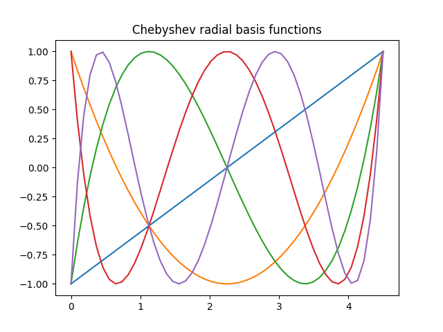
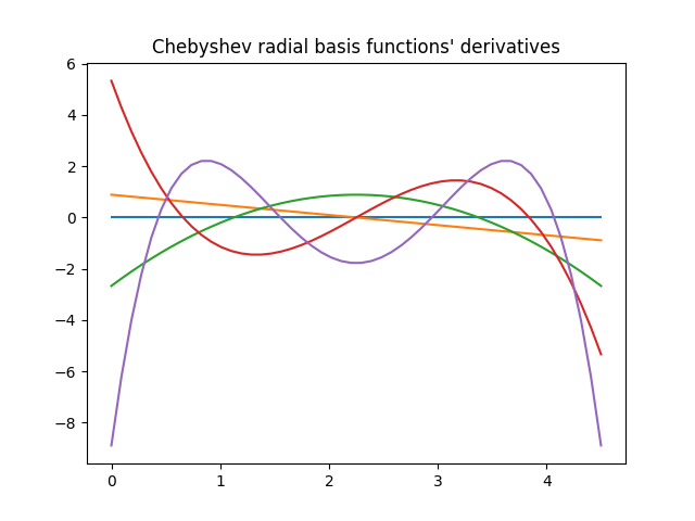
We can now look at the basis functions and their derivatives

radius = 4.5
basis = Chebyshev(max_radial=4, radius=radius)

r = np.linspace(0, radius)
for n in range(basis.size):
    plt.plot(r, basis.compute_primitive(r, n, derivative=False))

plt.title("Chebyshev radial basis functions")
plt.show()

for n in range(basis.size):
    plt.plot(r, basis.compute_primitive(r, n, derivative=True))
plt.title("Chebyshev radial basis functions' derivatives")
plt.show()

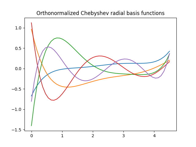
Before being used by featomic, the basis functions we implemented will be orthogonalized and normalized, to improve conditioning of the produced features. This is done automatically, and one can access the orthonormalized basis functions with the featomic.basis.RadialBasis.compute() method.

basis_orthonormal = basis.compute(r, derivative=False)
for n in range(basis.size):
    plt.plot(r, basis_orthonormal[:, n])

plt.title("Orthonormalized Chebyshev radial basis functions")
plt.show()

With this, our new radial basis definition is ready to be used with featomic.splines.SoapSpliner. This class will take the whole set of hyper parameters, use them to compute a spline of the radial integral, and give us back new hypers that can be used with the native calculators to compute the expansion with our custom basis.

spliner = SoapSpliner(
    cutoff=featomic.cutoff.Cutoff(
        radius=radius,
        smoothing=featomic.cutoff.ShiftedCosine(width=0.3),
    ),
    density=featomic.density.Gaussian(width=0.5),
    basis=featomic.basis.TensorProduct(
        max_angular=4,
        radial=Chebyshev(max_radial=4, radius=radius),
        spline_accuracy=1e-4,
    ),
)

hypers = spliner.get_hypers()

The hyper parameters have been transformed from what we gave to the featomic.splines.SoapSpliner:

print("hypers['basis'] is", type(hypers["basis"]))
print("hypers['density'] is", type(hypers["density"]))

hypers['basis'] is <class 'featomic.basis.Explicit'>
hypers['density'] is <class 'featomic.density.DiracDelta'>

And the new hypers can be used directly with the calculators:

calculator_splined = SphericalExpansion(**hypers)

As a comparison, let’s look at the expansion coefficient for formic acid, using both our splined radial basis and the classic GTO radial basis:

atoms = ase.build.molecule("HCOOH", vacuum=4, pbc=True)

calculator_gto = SphericalExpansion(
    # same parameters, only the radial basis changed
    cutoff=featomic.cutoff.Cutoff(
        radius=radius,
        smoothing=featomic.cutoff.ShiftedCosine(width=0.3),
    ),
    density=featomic.density.Gaussian(width=0.5),
    basis=featomic.basis.TensorProduct(
        max_angular=4,
        radial=featomic.basis.Gto(max_radial=4, radius=radius),
        spline_accuracy=1e-4,
    ),
)

expansion_splined = calculator_splined.compute(atoms)
expansion_gto = calculator_gto.compute(atoms)

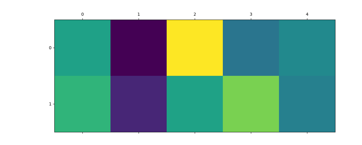
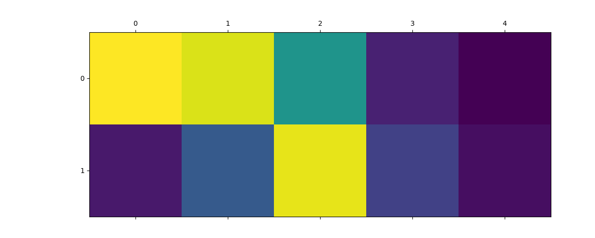
As you can see, the coefficients ends up different, with values assigned to different basis functions. In practice, which basis function will be the best will depend on the use case and exact dataset, so you should try a couple and check how they performe for you!

selection = dict(o3_lambda=0, center_type=8, neighbor_type=1)

plt.matshow(expansion_splined.block(selection).values.reshape(2, 5))
plt.matshow(expansion_gto.block(selection).values.reshape(2, 5))

• 
• 

<matplotlib.image.AxesImage object at 0x7f3b5e936cc0>

Since the calculation of the splines requires computing some integral numerically, the creation of the splines might take a while. After an initial calculation, you can save the splines data in JSON files; and then reload them later to re-use:

# convert the hypers from classes to a pure JSON-compatible dictionary
json_hypers = featomic.utils.hypers_to_json(hypers)

# save the data to a file
with open("splined-hypers.json", "w") as fp:
    json.dump(json_hypers, fp)


# load the data from the file
with open("splined-hypers.json", "r") as fp:
    json_hypers = json.load(fp)

# the hypers can be used directly with the calculators
calculator = featomic.SphericalExpansion(**json_hypers)

Finally, you can use the same method to define custom featomic.basis.ExpansionBasis and custom featomic.density.AtomicDensity; by creating a new class inheriting from the corresponding base class and implementing the corresponding methods. This allow you to create a fully custom spherical expansion, and evaluate them efficiently through the splines.